The datasets for EIS Data Compression (DC) factor investigation are chosen as follows:
1. search EIS study database to find out which study has adopted a specific compression scheme such as DPCM, JPEG95, etc. For example, study 29, 30, 31, 32, 91, 92, 142, 255, 258 have ever used JPEG90 compression scheme.
notes:
- study 29-32 are designed specially for all of compression schemes test, however, only study 29, 30 have generated useful fits files. Also the selection of compression scheme was done in eis_mk_study tool, rather than eis_mk_raster, thus there was no scheme information in these fits header. In this case one needs to manually find out the scheme for every fits files by study 29, 30.
- Some studies use multiple rasters (eg. study 142), for convenience of MDP data packets calculation the investigation only focuses on single-raster studies.
- Check the txt files study_summary.txt for more information about studies and their compression scheme selections.
2. Once knowing details (eg. ID) of rasters, which using a specific compression scheme, one can extract original data volume for these rasters (through EIS planning database), and the corresponding fits files (through EIS science database), then work out the data set for the investigation. The file datasets_list.txt lists the datasets used in this case.
notes:
- The datasets chosen here are out from EIS eclipse season
- In the 'plot' figures shown below, data points towards right-side of X-axis imply themselves coming from more recently observations.
The way to calculate EIS on-board compressed data volume with MDP status curves was described in previous post abut EIS DC factor: check it here.
The following links show DC factor variation in different scenarios (eg. AR, QS for SCI_OBJ, 1", 2", 40", and 266" for SLA).
A conservative estimation of average factor is indicated by orange dash-line on the plot, which could be used to improve EIS planning tools.
note:
EIS Data Compression (DC) factors listed here are only for Science Target & Slit/Slot selection. For factor variation upon exposure time, please refer H. Hara's 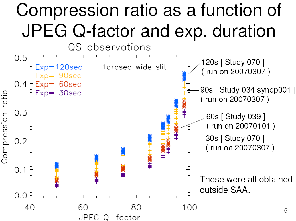 , (PDF)
For easy analysis a data table can be worked out as follows, using the plots shown in above links:
| Scheme | Total | QS | AR | CH | 1" | 2" | 40" | 266" |
|---|---|---|---|---|---|---|---|---|
| DPCM | 2.19 | 2.19 (2.38) | 2.19 | 2.19 | 2.54 | 2.46 | 2.19 | 2.18 |
| JPEG98 | 2.33 | 2.46 | 2.22 | 3.15 | 2.85 (avg) | 2.31 | 2.28 (2.32) | |
| JPEG95 | 3.26 | 3.64 | 3.26 | 6.12 | 6.38 (6.54) | 3.26 | ||
| JPEG92 | 3.63 | 3.31 (avg) | 6.65 (avg) | 2.74 (avg) | 6.53 (avg) | 2.74 (avg) | 3.63 (avg) | |
| JPEG90 | 3.82 | 3.82 | 4.34 | 3.73 | 4.67 (avg) | 3.84 | 3.78 | |
| JPEG85 | 4.51 | 4.82 | 4.51 | 4.91 | 3.9 (avg) | 4.51 | ||
| JPEG75 | 6.20 | 6.2 | 18.88 (avg) | 6.2 | 7.52 | |||
| JPEG65 | 7.33 | 19.94 (avg) | 25.97 (avg) | 7.33 (avg) | ||||
| JPEG50 | 17.72 | 20.98 | 17.72 | 35.37 (avg) | 17.72 |
Using DC factos (ie. 'total' in above table) to do trend fitting and compare wth those previous numbers used in EIS planning tool, we have:
total EIS DC factor:
| DPCM | JPEG98 | JPEG95 | JPEG92 | JPEG90 | JPEG85 | JPEG75 | JPEG65 | JPEG50 |
|---|---|---|---|---|---|---|---|---|
| 2.19 | 2.33 | 3.26 | 3.63 | 3.82 | 4.51 | 6.20 | 7.33 | 9.36 |
previous EIS DC factor:
| DPCM | JPEG98 | JPEG95 | JPEG92 | JPEG90 | JPEG85 | JPEG75 | JPEG65 | JPEG50 |
|---|---|---|---|---|---|---|---|---|
| 2.36 | 2.70 | 3.47 | 4.22 | 4.63 | 5.74 | 7.63 | 9.43 | 12.00 |
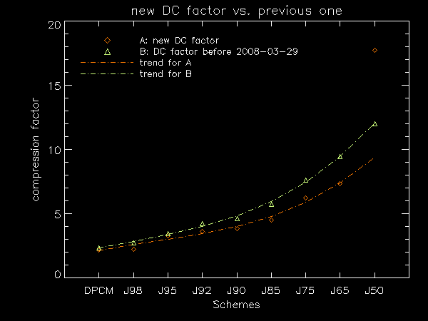 |
The orange dash-line in the figure can be described using equation: Y = 2.11768 + 0.556287*X - 0.0855122*X2 + 0.0161953*X3
Thus, the corresponding numbers on the line are:
| DPCM | JPEG98 | JPEG95 | JPEG92 | JPEG90 | JPEG85 | JPEG75 | JPEG65 | JPEG50 |
|---|---|---|---|---|---|---|---|---|
| 2.12 | 2.60 | 3.02 | 3.45 | 4.01 | 4.79 | 5.89 | 7.38 | 9.39 |
Which could be used by EIS planning tool as a simply improvment.
However in this calculation it looks that there is difference, but not too big, of compression factor in different scenarios, especially for example the DPCM compression (values are close to 2.19). This gives an idea we may use a set of single value of EIS compression factor for simplicity.
