EIS_XSTUDY#
About#
The eis_xstudy routine is actually a component of the EIS Planning Tool, and is used in both the construction of a timeline (eis_mk_plan) — to load something from the OSDB (official studies database) — and in eis_mk_study, used to select a study for modification in your own personal database before submission to the OSDB.To look at the OSDB, ensure that you have already run the command
print,fix_zdbase(/eis)
to instruct the planning tool to read from the OSDB. To look at your personal database instead (where you keep studies that you're designing) just replace /eis with /user in the above line.
Walk-through#
The eis_xstudy interface#
Below is an example of the widget that appears in SolarSoft when you type eis_xstudy:
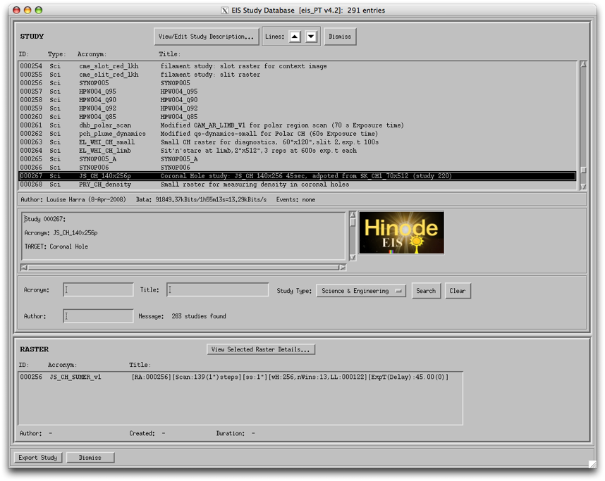 |
Study list#
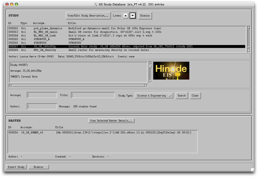
The top panel contains a list of all the studies in the database. I've cheated a little bit, in the sense that I've already scrolled down the list in the upper panel and chosen Study ID #267, the catchily-named JS_CH_140x256pAt the top of this widget there are two black triangular arrows. These can be used to reduce (down arrow) or increase (up arrow) the number of lines shown in the study list. (This can be especially useful if your screen is a lot smaller than the default widget size.) This looks like so:
 |
There's also a button at the top of the widget marked View/Edit Study Description. I'll come back to that in a while.
Information bar#
In the status bar immediately beneath the study list is a sort of information bar: here you can see important information such as the amount of data that the study is expected to generate in kbits (this is approximate, since compression factors vary a little from dataset to dataset), the duration in hours minutes and seconds (fixed, but with a little margin added), and the consequent rate of telemetry from EIS to the Hinode Data Recorder (DR).The volume here is probably one of the most important factors, since it determines how many times (if any!) a study can be run during an OP Period — see SbandObservingInfo for what this means in practice.
Study description area#
Below this information bar, there's a text area that contains the Study Description. This is information which the study author has included, indicating what they originally intended the study to be used for One of the nice things about EIS is that you can recycle a study already designed by someone else for a similar — or even different — purpose, without having to go through this design step.To read the study description in full, either scroll down this panel with the scroll bar, or go the the button at the top marked View/Edit Study Description (I told you I'd come back to it). This opens up a window like this:
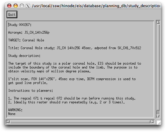 |
As you can see, the study contains information for the person using this study, if it is to be used for the original proposal.
There is also often information in the study description added by the study validator, the person who tests the study on the EIS demonstration model at MSSL, before it enters the OSDB. This information can include things like warnings — e.g., information about how not to use the study — and so on.
To get rid of this window, just click on Quit.
Search methods#
If you have some idea about the study you're looking for, e.g. it has EL in the name, or it was written by George Doschek, you can use the search facility to save you time.Below the Study Description panel, you can search on one or more fields, namely Acronym (the name of the study), Title (confusingly, a description of the study), or Author (self-explanatory). Since I've mentioned George Doschek, let's try a search for studies he's designed. I don't know any other Doscheks on the EIS team, so I'll just use his surname:
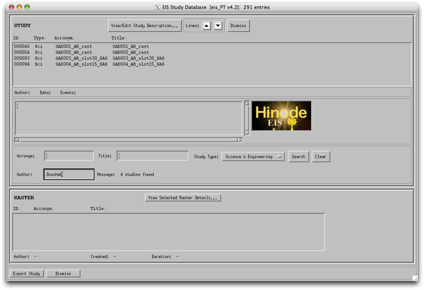 |
You can see that this results in four studies showing up, each of which was authored by someone called Doschek.
You can clear the search fields by clicking Clear on the right-hand side.
Changing the Study Type drop-down list on the right from Science & Engineering to Science excludes all engineering-type studies from our search (although this tends to be more useful when looking for specifice engineerings studies hidden amongst the forest of science studies).
Raster panel#
Below the search area is the Raster panel, where you can start to look at the details of the study's execution. Let's take another example to look at this.
For the purposes of this example, my memory's a bit shaky, so I just remember that the study I'm interested in has the letters CH in the acronym. Searching for these letters in the Acronym field produces these results:
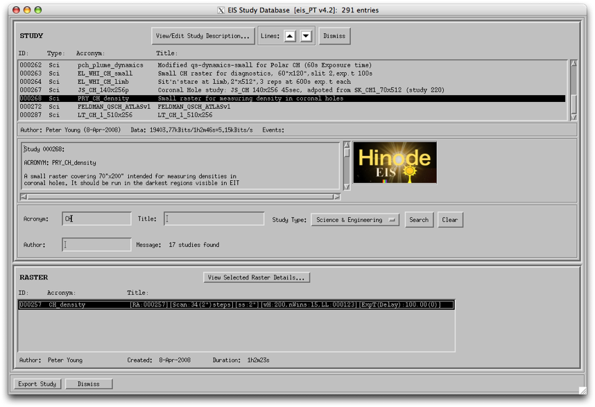 |
This also makes the raster panel go from being empty to showing the rasters in the selected study (if no study is highlighted, eis_xstudy can't know which rasters to display).
A study is essentially a package: it's an observing programme that contains a pre-defined order of executable rasters. eis_xstudy allows you to look inside this package, at the rasters that a study contains, as well as the details of those rasters. You'll see that Study #268 PRY_CH_density contains raster ID #257 CH_density. In most practical cases, studies contain only one raster. But the study is what is actually makes it onto the timeline (schedule) for EIS.
It's important not to confuse raster and study IDs when requesting observations. Please always use the Study ID or full study acronym.Viewing raster details#
If we want to see what happens when PRY_CH_density runs, the best thing to do from here is to click on each raster in the raster panel (in this case, there's only one), and then click the View Selected Raster Details... button just above.This opens up a separate window which details how the raster will execute on-board the space-craft (only omitting pointing details, which are flexible). The window should look something like this:
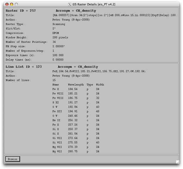 |
This is also a two-panel window. The reason for that is that, similar to the way that a study can't exist without a raster, a raster can't exist without a line list. More on that later...
The upper panel here shows the key information that we need to know about to describe the raster, namely:
| Parameter Name | value |
|---|---|
| Title | to be discussed later |
| Author | Peter Young |
| Raster Type | Scanning |
| Slit/Slot | 2" |
| Compression | DPCM |
| Window Height | 200 pixels |
| Number of Raster Pointings | 34 |
| FM Step Size | 2.0" |
| Number of Exposures/step | 1 |
| Exposure time(s) in seconds | 100.0 |
| Delay times (ms) | 0.0 |
So, what to do with all this information? Let's put it in context.
Author
The author of this raster is Peter Young. Fairly easy
Raster Type
The term raster usually conjures up the idea of a rectangular image. And that's what EIS does when it makes its observations. It's just that in some cases the X dimension is time, rather than space.
EIS has two modes of raster. The first is scanning raster, which is what we see in this example. EIS takes a restricted-field image of the Sun and then disperses it, perpendicular to the length of the slit. Then, a fine mirror (FMIR) adjusts the X position on the Sun where that image comes from (by the amount indicated in FM Step size) and makes another image. This is how EIS builds up spectroheliograms (spectral image of the Sun).
The second mode is the so-called fixed slit or sit'n'stare raster type, whereby the same slit or slot-size portion of the Sun is repeatedly made into an image and dispersed. This is qualitatively the same as the scanning raster, except for the fact that we are usually more interested in the time-dependent changes at a particular location.
Slit/Slot
a.k.a. SLA — SLit/slot Assembly
EIS makes images of different widths every time it takes an exposure (and disperses it). Slit spectra contain direct spectroscopic information, but take time to build up information over areas (see Raster Type above). To make slit spectra, EIS uses two slits: 1" and 2" in width.
The 1" slit has less spatial coverage (because it is narrower) so there is sharper spectral resolution; meanwhile, the advantage of the 2" slit is that it is twice as wide, and thus it can accumulate photons twice as quickly as the 1" slit. (Note that this argument does not extend linearly to the width of the slots). For more image-based information, at the expense of line profile information, we can make slot images (scanning or sit'n'stare). In both cases the images are dispersed on the detector. The slot images are a sort of convolution of a spectrum with an image. However, the narrow slot — 40" wide — has been chosen so that essentially monochromatic images of the Sun can be made in many lines, without significant blending with images made in nearby lines.
The width of the wider slot — 266" — was chosen for ground calibration reasons, rather than scientific considerations. However, the Fe XV line at 284 Å is sufficiently removed from other active region lines that we can essentially make images of only Fe XV in bright coronal loops. In other lines, the images resemble the overlappograms produced by the Skylab S020 spectrograph (see Figure 2 of http://solar.physics.montana.edu/reiser/ for a full-Sun idea of what this means), though with smaller spatial extent.
Compression Type
In order to make the process of transferring data to the ground more efficient, data from all Hinode instruments can be compressed on-board the spacecraft by the mission data processor or MDP.
The MDP allows several choices of compression:
| Scheme | Compression Type |
|---|---|
| Uncompressed | None |
| DPCM | Lossless |
| JPEG98 | lossy (Q factor 98) |
| JPEG95 | lossy (Q factor 95) |
| JPEG92 | lossy (Q factor 92) |
| JPEG90 | lossy (Q factor 90) |
| JPEG85 | lossy (Q factor 85) |
| JPEG75 | lossy (Q factor 75) |
| JPEG65 | lossy (Q factor 65) |
| JPEG50 | lossy (Q factor 50) |
In addition to these webpages showing the more involved analysis results, the current values used for DC factors in making observations are stored in $SSW/hinode/eis/idl/spacecraft/decompression/eis_get_compression_factor.pro
Window Height
Whereas the width of each spectral window can vary (see Line Lists below), the height of the image ysize read out from the CCDs is necessarily fixed for each window. So each raster has the same height in all spectral windows. This height is expressed in arcseconds. In EIS's design, it was decided that a 512" image height would be sufficient (1 pixel = 1"), so this is the maximum image height that can be made at any one time.
Number of Raster Pointings
Scanning raster-specific
This is a little confusing, but it tells you the number of times N that the mirror must move between observations to build up a scanning raster, i.e. 1 less than the number of positions at which EIS makes an exposure.
Working out the size of a raster
If N+1 is the number of positions at which the slit makes an image, Σ texp is the sum of the exposure times (usually there is only one) at each position (in seconds), and xstep is the size (in arcseconds) of the step, then it takes n × Σ texp × xstep seconds to build up a spatial image of an area that is xsize = ( (n × xstep) + SlitSize ) arcseconds across.
Putting this together with the xsize, worked out above, tells you the spatial extent of the observation that this raster produces.
Exposure Times
EIS allows its user to make more than one exposure at each position on the Sun, and these exposures can have independent shutter-open times. In fact, you can have up to eight such exposures at each fine mirror position.
Delay Times
Delay times can be up to 655.35 seconds long (2^16 -1 × 10-ms units), and come after each exposure. The number of delay times has to be the same as the number of exposure times, but typically these delays are set to zero.
For example, with two exposure times of 10 and 120 seconds, and delays of 100 seconds and 200 seconds, a typical ordering of events could go like this:
| Event |
|---|
| Move fine mirror to starting position |
| Take an exposure for 10 seconds |
| Read out exposure |
| Delay for 100 seconds |
| Take an exposure for 120 seconds |
| Read out exposure |
| Delay for 200 seconds |
| Take an exposure for 10 seconds |
| Read out exposure |
| Delay for 100 seconds |
| Take an exposure for 120 seconds |
| Read out exposure |
| Delay for 200 seconds |
| Move fine mirror to next position |
| etc. |
Raster Title
Knowing what all the above information means, you can also get a quick idea of most of the characteristics of a raster from the single-string raster Title field in eis_xstudy.
This "summary", if you like, is composed of a series of square-bracketed terms in the following order:
| RA:RasterID |
| Scan:NumberOfPositons-1(SizeOfStep)steps, |
| ss:SLAchoice |
| wH:WindowHeight,nWins:NumberOfSpectralWindows,LL:LineListID |
| ExpT(Delay):ExpTimeNumberOneInSeconds(DelayNumberOneInHundredthsOfASecond), ... |
and can be handy when you understand how it works, because it means you don't need to delve into the raster description to find out how large it is, which slit or slot it uses, how long the exposure times(s) is/are, etc.
Note that since engineering studies are created by hand, rather than through the planning tool, it's not normally possible to view their contents (such as number of exposures, or exposure time) in the Raster panel.
Line List#
The most critical part of the raster description that isn't summarised in the Raster Title is the Line List. This is because the line list is too variable to easily summarised. So, it gets its own panel in the raster description.Note that, like studies and rasters, line lists have and ID and acronym.
Rationale of a Line List
When EIS makes a spectral image of a slit- or slot-sized portion of the Sun, it exposes the whole of both detectors, which amounts to some 2 × 2048 × 1024 pixels. At 16 bits per pixel (2 reserved for marking which half of which detector a pixel belongs to), this would create a massive 8 MB for all data from the detector, at each position on the Sun!
So, in order to limit telemetry need — even before the transition to the S-band antenna — EIS was designed so that only the spectral portions of interest on the detector would be telemetered to the ground for a given observation.
Line lists are described in terms of absolute wavelength, according to the standard wavelength calibration, so you don't need to work things out in terms of pixel co-ordinates.
Title
You'll see that, like the raster, a Line List has a one-line so-called Title string associated with it. Since this is truncated, it doesn't serve much purpose, and we'll skip it here.
Author
Again, fairly self-explanatory
:-)
One point to perhaps reiterate, though, is that you can use a line list created by anyone else in your study. All line lists, rasters, and studies in the OSDB are there to be re-used and cannibalised by anyone wanting to propose an observation.
Number of lines
There can be up to 25 spectral windows in a line list, but the minimum is normally three: the core lines. The core lines are
| Ion | Wavelength (Å) |
|---|---|
| Fe XII | 195.12 |
| Ca XVII | 192.82 |
| He II | 256.32 |
Line List Detail
Each spectral window can have a width that is an integer multiple of 8, from 8 to 1024 (half a CCD width), and there can be up to 25 windows, each with independent widths. In the example image above, you can see that most windows have a width of 24 pixels (a little over 0.5 Å), which is usually adequate. But a few windows are wider (32, 40 or 48 pixels). Wider windows often (but don't necessarily) indicate that the line list author was trying to capture other lines by using a wider spectral window.
This also helps to explain why the core lines of Fe XII (195.12 Å) and Ca XVII (192.82 Å) aren't explicitly included in this line list: they are already covered by the Fe XII window at 194.91 Å and the O V window at 192.84 Å, respectively.