A challenge with EIS
The Sun is the only star whose fine structure can be
observed from the Earth.
Resolving the structure and dynamics of the solar corona is crucial for
understanding energy release processes such as flares.
Due to this, the resolution of solar telescopes has
been continually improving.
However, there is a problem: a good measurement requires a good
reference point.
EIS has a high resolution but turned out to be very
sensitive to a deformation caused by instrumental
temperature variation.
This is seen as a spectrum drift on the detector
caused by the optical path inside the EIS deviating
by 0.01 mm.
The spectrum drift makes it difficult to define a wavelength reference,
which is essential for deducing a Doppler velocity.
The top panel in
Figure 1 shows the spectrum position on the detector
over time.
The instrumental drift amounts to 70 km/s in Doppler velocity scale and
this must be corrected
to measure a precise Doppler velocity in the corona.
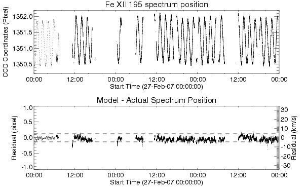
Figure 1:
The top panel shows the spectrum position on the detector over time;
The bottom panel shows the error of the ANN model estimation of EIS instrumental drift (≤ 5 km/s)
Deriving an empirical law from past observations
The temperatures of EIS are regularly monitored, but it is not
an easy job to build a realistic thermal model of the instrument from
this data.
There is a sophisticated method called an artificial neural network (ANN),
which can deduce an empirical relationship between input and output
without a detailed knowledge about the principles behind them.
The strategy is simple; find an empirical relationship between
temperature and spectrum drift. Fortunately, EIS has obtained
plenty of data during its 3.5 three years in orbit.
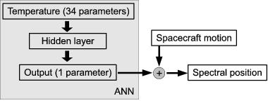 Figure 2: a schematic diagram of the ANN method
Figure 2 shows a schematic diagram of the method followed. The ANN, or a
black box, was
optimized to reproduce the spectrum drift from the temperatures.
If the model works, a wavelength reference can be defined by
using instumental temperatures.
Does it really work? The bottom of
Figure 1 presents the error
of the model estimation, which is normally smaller than 5 km/s.
The spectrum drift is effectively suppressed by this method.
How it works
A good method must be tested against real observations.
Figure 3 shows an active region close to the west limb.
It indicates a significant flow in a coronal loop after a flare.
It also shows a sign of an outflow from the dark periphery of the
active region, which has been studied in many publications.
So far, a velocity averaged over an observing region has been
regarded as a reference.
In some cases, however, the assumption of null velocity is
not valid, particularly when high speed flows are expected.
One of the advantages of our method is that it is independent
of observing sequence as it only requires instrumental
temperatures.
This method is provided as a part of the Solarsoft.
Instructions on EIS data preparation are provided on
EIS Wiki (
/eiswiki/).
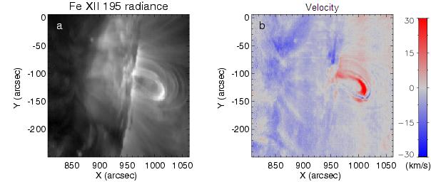
Figure 3:
The method is applied to EIS real observations on December 17, 2006
References:
This article is based on a paper:
S. Kamio, H. Hara, T. Watanabe, T. Fredvik, and V.H. Hansteen 2010 Solar
Physics, in press
or arXiv:1003.3540 (http://arxiv.org/abs/1003.3540)