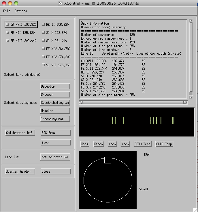
The Xcontrol window may be decsribed as the QL main control window for the selected raster. From this window the user is presented with some basic information about the raster, and the basic displays are selections available from here.
 |
- Display header: Launches a text window displaying the contents of the header.
- Compare EIS/Chianti spectra: This is used to compare an average EIS spectrum calculated from the raster with a Chianti spectrum of the same wavelength region. An intermediate window pops up where the user must select the proper emission measure for the Chianti spectrum. The Chianti spectra have been pre-calculated for the EIS wavelength regions and the most relevant emssion measure regimes. The Chianti spectra are stored in proper files and distributed as a part of the EIS QL package.
The first box in the left column lists the line windows contained in the raster, with the short wavelength band to the left and the long wavelength band to the right, as well as line window information when available (from the planning tool). The line window selection is relevant for all display modes except the detector display, where full CCD images are displayed.
The second box in the left column is used to select display mode.
- The detector display shows full CCD images (see the Xdetector section below), i.e. count rates as a function of wavelength (abscissa) and slit position (ordinate). The ordinate translates into Solar-Y position.
- The browser allows the user to browse the various line windows and line profiles.
- The spectroheliogram display shows count rates for the selected line(s) as a function of wavelength (abscissa) and slit position (ordinate), one imager for each selected line and exposure.
- The xwhisker mode shows launches one separate display window for each selected line. Here, the line countrates are displayed as a funtion of wavelength (abscissa) and exposure number (ordinate), which translates into time or raster position. If the raster is a sit-and-stare, the ordinate axis translates into time, if it is a scanning raster, the it is Solar-X coordinates.
- The last display mode available from Xcontrol is intensity map. It displays data from one line window as a function of exposure number (abscissa) and slit position (ordinate). In order to do this, an average over the line profile (wavelength) has been calculated. Again, the abscissa dimesnion will be Solar-X for a scanning raster and time for a sit-and-stare.
The third box allows the user to invoke eis_prep; which will be run in default mode once the "EIS Prep" button is pressed. (The "Calibration Def" button currently serves no useful purpose.)
The fourth box in the left hand column allows one to do a quick line fit of the lines selected above, and to view the resulting image, velocity, and width maps.
In the right column, there is a text window (not editable) that presents key parameters describing the raster, such as if it is a sit-and-stare or scanning raster, number of exposures, number os slit positions etc.
Below this you will find a mini display showing the first exposure in the raster on both detectors.
There follow five buttons that will display information on the x-position of the exposures in the raster, the position of the x- and y- center of the FOV, and the CCD temperatures during the observation.
Finally, at the bottom of the right column we find a display indicating the position of the raster on the Sun and a number of acronyms which indicate what level the data is prepped to. It also indicates whether or not the data, as modified by the QL-software, has been saved or not.
