EIS_GETWINDATA - a wrapper to the EIS objects#
The EIS data are stored in IDL objects, and all information about the data can be accessed through object methods. However, sometimes it is convenient for the user to dump a particular wavelength window to an IDL structure, together with useful information such as pointing coordinates, start time, exposure time, etc.
The routine that does this is called eis_getwindata and an example of how to call it for the Fe XII 195 data window is given below.
IDL> d=eis_getwindata('eis_l0_20070202_104212')
% EIS_GETWINDATA: no window number input, select one . . .
iwin line_id wvl_min wvl_max
0 FE X 174.530 174.36 174.70
1 FE X 175.260 175.10 175.43
2 O VI 184.120 183.95 184.29
3 FE X 184.540 184.38 184.71
4 FE VIII 185.210 185.05 185.38
5 FE XII 186.880 186.72 187.05
6 FE XI 188.230 188.06 188.39
7 CA XVII 192.820 192.65 192.98
8 FE XII 193.510 193.34 193.67
9 FE XII 195.120 194.94 195.28
10 FE XIII 202.040 201.87 202.21
11 FE XIII 203.830 203.65 203.99
12 HE II 256.320 256.15 256.49
13 FE XVI 262.980 262.83 263.17
14 FE XIV 264.780 264.63 264.97
15 MG VI 268.990 268.84 269.17
16 FE XIV 274.200 274.05 274.38
17 SI VII 275.350 275.20 275.54
18 O IV 279.930 279.78 280.12
19 FE XV 284.160 284.01 284.34
Select a window to read [0...19]> 9
IDL> help,/str,d
** Structure <2974204>, 19 tags, length=8397328, data length=8397322, refs=1:
FILENAME STRING 'eis_l0_20070202_104212.fits.gz'
LINE_ID STRING 'FE XII 195.120'
INT FLOAT Array[16, 256, 256]
ERR FLOAT Array[16, 256, 256]
WVL DOUBLE Array[16]
TIME FLOAT Array[256]
TIME_CCSDS STRING Array[256]
EXPOSURE_TIME FLOAT Array[256]
SOLAR_X FLOAT Array[256]
SOLAR_Y FLOAT Array[256]
NL LONG 16
NX LONG 256
NY LONG 256
SCALE FLOAT Array[2]
UNITS STRING 'DN'
MISSING INT -100
IWIN LONG 9
HDR STRUCT -> <Anonymous> Array[1]
TIME_STAMP STRING 'Fri Jul 6 08:44:52 2007'
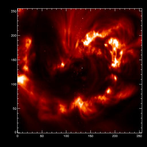
IDL> plot_image,sigrange(total(d.int,1))
The resulting image is below. The routine also works on level1 data processed with eis_prep. More information is available in the header.
 |
PLOT_EIS_RASTER - plotting data from eis_getwindata#
I have done a small program "plot_eis_raster.pro " where you can visualize the structure with the coordinates, time and name of the window.
plot_eis_raster.pro is just valid for the slit rasters (I haven't tried with any slot).
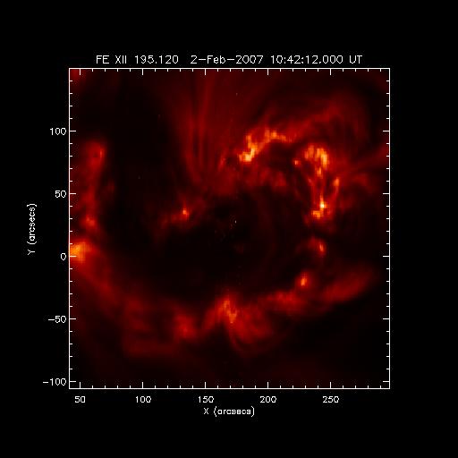
A few comments: the time that it shows is the time of the beginning of the raster; and the coordinates is calculated using the mean value of d.solar_x and using the size of the slit per each pixel. To use it you just have to (for the same example than before):
IDL> plot_eis_raster,d
 |
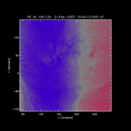
Or if you want to change the value to plot (e.g. the values that you obtain after fit the line)
To plot the array called velocity (in my case velocity=reform(result(1,*,*)) ):
IDL> plot_eis_raster,d,value=velocity
 |
Also you can use all the keywords of plot_map (dmin, dmax, etc.)
And you can save the map produced,
IDL> plot_eis_raster,d,value=velocity,map=velocitymap
-David Pérez-Suárez, 06 Jul 2026
Operations on WINDATA structures#
There are a number of routines available for performing operations on WINDATA structures. The full set are listed in EIS Software Note #21.
Spatial binning (EIS_BIN_WINDATA)#
Sometimes it is useful to perform spatial binning on EIS data in order to improve photon statistics on the emission lines. The routine eis_bin_windata is available in Solarsoft which takes the output from eis_getwindata and performs binning in the X and/or Y directions while preserving the form of the eis_getwindata structure. Errors on the intensities at each of the binned pixels are correctly calculated.
The routine is called as, e.g.,
IDL> wd=eis_getwindata(l1name,195.12)
IDL> wdnew=eis_bin_windata(wd,xbin=2,ybin=2)
Joining two WINDATA structures (EIS_JOIN_WINDATA)#
Takes two WINDATA structures from a data-set and joins them in the wavelength dimension to produce a single, new WINDATA structure. This is most useful if the two WINDATAs are directly adjacent on the detector.
IDL> wd1=eis_getwindata(l1name,184.54)
IDL> wd2=eis_getwindata(l1name,185.12)
IDL> wd=eis_join_windata(wd1,wd2)
Correcting data arrays for orbit variation and slit tilt (EIS_SHIFT_SPEC)#
The wavelength scale for individual spatial pixels changes across the raster due to the thermally-induced, orbital drift of line centroids and the EIS slit tilt. The routine EIS_SHIFT_SPEC takes an array of wavelength corrections, and interpolates the intensity and error arrays such that the same wavelength scale applies to each spatial pixel. Due to complications of interpolating over missing pixels, the /refill option should be used in the call to eis_getwindata.
IDL> eis_wave_corr_hk, l1name, wvl_corr
IDL> wd=eis_getwindata(l1name, 195.12, /refill)
IDL> wd_new=eis_shift_spec(wd,wvl_corr)
Trimming the wavelength range of a windata structure (EIS_TRIM_WINDATA)#
This routine is intended for WINDATA structures with a large wavelength coverage; most commonly this will be full CCD data. An example use is when EIS_AUTO_FIT is to be run on just a single emission line within a full CCD spectrum. By trimming the wavelength coverage of WINDATA to just including the wavelength region around the line of interest, the spectrum becomes easier to fit. The usage is as follows for the case where Fe XII 195.12 is to be studied:
IDL> wd=eis_getwindata(l1name, 195.12, /refill)
IDL> wd195=eis_trim_windata(wd,[194.12,196.12])
Here a +/- 1 angstrom band around the line of interest is extracted.