Elemental Abundances at Coronal Hole Boundaries as a Means to Investigate Interchange Reconnection and the Solar Wind

 

Introduction
Coronal holes (CHs) are known sources of the fast solar wind, characterized by 'open' magnetic field lines. However, at the coronal hole boundary (CHB) region, there is a transition from the open field lines in CHs to the closed fields lines in the quiet Sun. At this boundary, previously confined plasma from quiet Sun loops can be released into interplanetary space through interchange reconnection with the open magnetic field of the CH, creating a potential source of the observed slow solar wind. As an observational signature of the interchange reconnection, we have used the ratio of low first ionization potential (FIP) elements to a high FIP element (i.e., the FIP bias). Low FIP elemental abundances are enhanced in closed loops as compared to high FIP elements. Moreover, the CHB region may contain more open flux than previously thought, offering a potential solution to the longstanding "open flux problem". Our study leverages spectroscopic observations of elemental abundances at CHB regions to constrain interchange reconnection models and examine the contribution of these regions to the solar open flux budget.

Observations and analysiss
Our analysis was focused on raster observations using the 2" slit of EIS on 2016 March 25. The field of view (FOV) was centered on an equatorial coronal hole and included a portion of the quiet Sun on either side of the CH (see Figure 1). The FIP bias was derived using a differential emission measure (DEM) analysis (C. Guennou et al. 2015) and a linear combinations ratio (LCR) method (N. Zambrana Prado & Buchlin 2019). For both methods Iron and Silicon were used as the low-FIP elements; Sulfur was used as the high-FIP element. To investigate the change in the FIP-bias values as we go from the coronal hole to the quiet Sun, we took longitudinal cuts across the coronal hole and studied the FIP bias as a function of distance from the CHB. The FIP-bias values along the cut were smoothed to clarify any trends with distance from the CHB. A single longitudinal cut can be seen in Figure 1.

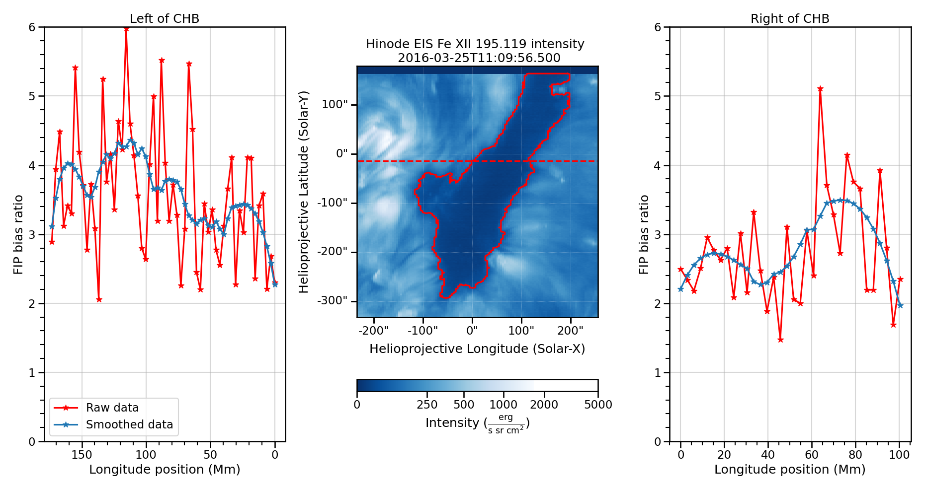
Figure 1: FIP-bias along a longitudinal cut across the coronal hole. Left: FIP-bias data as a function of position along the longitudinal cut for the left side of the coronal hole boundary. Center: The intensity of the Fe XII line including the calculated CHB (red line). The red dashed line represents the longitudinal cut shown in the side panels. Right: FIP-bias data as a function of position along the longitudinal cut for the right side of the coronal hole. For the outer left and right plots, zero in the x-axis represents the location where the longitudinal cut intersects the CHB to the left and to the right, respectively.

The behavior of the FIP bias close to the coronal hole exhibits variability among longitudinal cuts. This stems mostly from the existence of different features along each cut. To address this variability, we focused on identifying the overall trend of the FIP-bias values as we approach the CHB, from each side. We began by selecting from the smoothed FIP-bias data all longitudinal cuts that intersected the coronal hole within our FOV. These longitudinal cuts were then divided into two parts, one corresponding to the left side and the other to the right side of the coronal hole, as is shown in Figure 1. Next, we aligned both portions of all longitudinal cuts with the corresponding left or right edge of the coronal hole. We then averaged the FIP-bias values as a function of distance away from the coronal hole, for both sides. The results of the average FIP bias as a function of distance for both sides of the coronal hole, are shown in Figure 2.

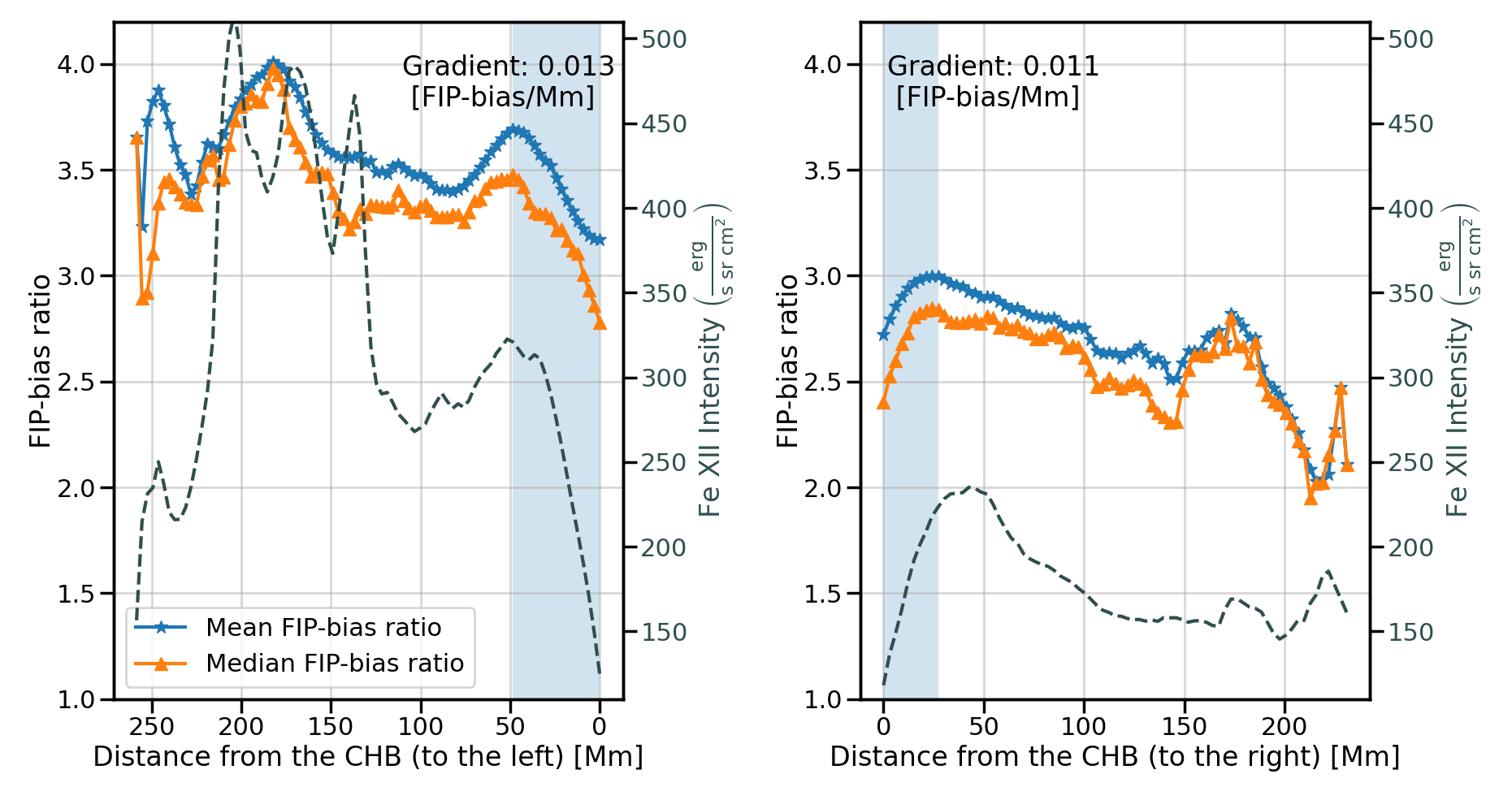
Figure 2: Average FIP bias as a function of distance (in longitude) from the CHB. The blue shaded regions indicate where the interchange reconnection is inferred to occur. The FIP-bias values shown here were derived using the DEM method. The dashed line indicates the average intensity of the Fe XII line.

Results
Our results reveal that the CHB region has a width of 30 to 60 Mm, which is comparable to the ≈30 Mm size of supergranules. We found that the CHB width was slightly larger for the left side of the coronal hole compared to the right, for both methods (DEM, LCR), but this variation was not significant.

• Open flux diffusion coefficient: We estimated the diffusion coefficient (κ) of the open flux diffusion model (L. A. Fisk & N. A. Schwadron 2001) using the properties of the average FIP bias in the CHB region. We found that κ = 1.3 ± 0.6 × 10¹⁴ cm² s^-1 at the CHB region. This lies between the theoretically expected values for CHs and quiet Sun. Following the assumptions of L. A. Fisk & N. A. Schwadron (2001), the derived diffusion coefficient suggests that smaller loops with heights of ∼30-60 Mm facilitate the interchange reconnection at the CHB region. It is possible that larger loops (>=200 Mm) also contribute to the interchange reconnection at the CHB region, but any observable signature lies outside our FOV.
• Additional open flux: Our FIP bias results indicate that there are opening and closing magnetic field lines in an area ∼30-60 Mm wide next to the coronal hole. Consequently, there is an amount of diffused open flux in this area. Remote sensing estimates of the open flux usually account only for the visibly dark CH areas (in EUV), neglecting any contribution from these brighter CHB regions. By projecting the CHB region on a line-of-sight magnetogram (Figure 3) we were able to derive a first-order estimate of the open flux present in this extended boundary area. Our results suggest that the CHB region contains ∼37%-71% of additional open flux compared to the CH alone. Our estimates of this, previously unaccounted, open flux do not appear to be sufficient to reconcile the difference with the in-situ calculations, but they help to reduce the gap and may point to a resolution for the open flux problem.

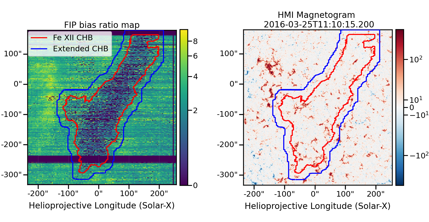
Figure 3: The CHB and the extended CHB. Left: FIP-bias map with contours showing the CHB from Fe XII in red and the extended CHB in blue, for a CHB width of 30 Mm. Portions of our FOV, where the data are corrupted, have been set to zero and are visible as dark strips. Right: LOS HMI magnetogram aligned with the EIS FOV and with the same contours. .

For more details, see:
Koukras et al., 2025, ApJ, 982:173:
Elemental Abundances at Coronal Hole Boundaries as a Means to Investigate Interchange Reconnection and the Solar Wind


References
Fisk, L. A., & Schwadron, N. A. 2001, ApJ, 560, 425
Guennou, C., Hahn, M., & Savin, D. W. 2015, ApJ, 807, 145
Zambrana Prado, N., & Buchlin, E. 2019, A&A, 632, A20

 

For more details, please contact: Dr. Deb Baker.

Prev

Archive

Next

Next EIS Nugget    »»  coming soon...

TBC