Searching for evidence of subchromospheric magnetic reconnection on the Sun
Deb Baker (UCL/MSSL)

Within the coronae of stars, abundances of those elements with low
first ionization potential (FIP) often differ from their photospheric
values. The coronae of the Sun and solar-type stars mostly show
enhancements of low-FIP elements (the FIP effect) while more active
stars such as M dwarfs have coronae generally characterized by the
inverse-FIP (I-FIP) effect. Highly localized regions of I-FIP effect
solar plasma have been observed by Hinode/EIS in a number of large, highly
complex active regions, usually around strong light bridges of the
umbrae of coalescing/merging sunspots. These observations can be
interpreted in the context of the ponderomotive force fractionation
model which predicts that plasma with I-FIP effect composition is
created by the refraction of waves coming from below the plasma
fractionation region in the chromosphere. A plausible source of these
waves is thought to be reconnection in the (high-plasma beta)
subchromospheric magnetic field. We use the 3D visualization technique
of Chintzoglou & Zhang (2013) combined with observations of localized
I-FIP effect in the corona of AR 11504 to identify potential sites for
subchromospheric reconnection and and we search for its possible consequences in the solar
atmosphere such as upflows and heating.
Hinode EIS/Observations
AR 11504 was a large, highly complex active region with multiple episodes of significant flux emergence and sunspot rotation leading to persistent flaring and CME events (James et al. 2017, 2020). Hinode/EIS observed the active region from 13-15 June 2012 during which time, I-FIP plasma was observed at the tail end of the decay phase of an M1.9 class flare on 14 June and during the peak of a C3.0 class flare on 15 June. Two line intensity ratios were used to detect the I-FIP plasma: 1. high-FIP Ar XIV 194.40 A/low-FIP Ca XIV 193.87 A for 4 MK plasma and 2. high-FIP Ar XI 188.82 A/low-FIP Fe XIV 264.79 A for 2 MK plasma. In addition, the intermediate-FIP S (sulfur) was included in the analysis because its behavior provides insight into the height of the plasma fractionation in the chromosphere. In the upper chromosphere/transition region, S acts like the noble gases with very high FIP and in the low chromosphere, it behaves as a low FIP element. See Figure 1.
Regions of I-FIP plasma are observed on the eastern side of AR 11504 for June 13 and 14 in both the Ar XIV/Ca XIV and Ar XI/Fe XIV ratio maps. On 15 June, localized I-FIP plasma is observed on the western side of the AR at 2 MK but not at 4 MK. There the plasma has evolved to photospheric composition in the Ar XIV/Ca XIV ratio map. Interestingly, in the Ar XI/Fe XIV ratio map, I-FIP plasma appears to extend along loops to the south/southwest.
Where the intermediate-FIP S XIII and XI ions are used in the ratio maps instead of the low-FIP Ca and Fe ions, S behaves like a low-FIP element on June 13 and 14, especailly in the Ar XIV-Ca XIV maps throughout the core of the AR. S is less fractionated in terms of both degree and spatial extent when comparing the lower temperature Ar XI-S XI and the higher temperature Ar XIV-S XIII ratio maps.
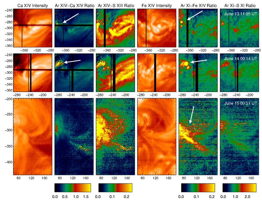
Figure 1: Hinode/EIS observations of AR 11504 for 13 June 2012 at 11:05 UT (top), 14 June at 00:14 UT (middle) and 15 June at 00:51 UT (bottom). Observations on 13, 14 June are of the AR's following (negative) polarity and then of the leading (positive) polarity on 15 June. Left to right: Ca XIV 193.87 A intensity map, Ar XIV 194.40 A/Ca XIV 193.87 A and Ar XIV 194.40 A/S XIII 256.69 A line intensity ratio maps, Fe XIV 264.79 A intensity map, Ar XI 188.82 A/Fe XIV 264.79 A and Ar XI 188.82 A/S XI 188.68 A line intensity ratio maps. In color bar of the ratios, I-FIP regions are in yellow, photospheric composition is approximately orange and coronal composition is green/blue.
The specific locations of the I-FIP plasma within AR 11504 are shown in Figure 2 with SDO/HMI magnetic field, HMI continuum, SDO/AIA 1600 A, and reverse-color AIA 94 A maps. The contours of I-FIP plasma from the EIS scans of Figure 1 are overplotted on the SDO/HMI and AIA maps. Pink/blue contours and arrows correspond to I-FIP patches in the Ar XI-Fe XIV / Ar XIV-Ca XIV line ratio maps.
On the eastern side of AR 11504, patches of I-FIP plasma are observed in the negative polarity fragments forming the southern of the two following sunspots. This is the location of the large scale flux emergence that occurred from 11-15 June. In the leading (positive) sunspot, the I-FIP plasma lies above the strong light bridge separating the large pre-existing spot and a smaller spot rotating around it that results from new flux emergence. Both sites are associated with the footpoints of the flaring loops spanning the AR and repeated flare ribbon crossings of the coalescing leading and following sunspots. The locations of I-FIP plasma in AR 11504 are consistent with previous studies (Baker et al. 2019, 2020).
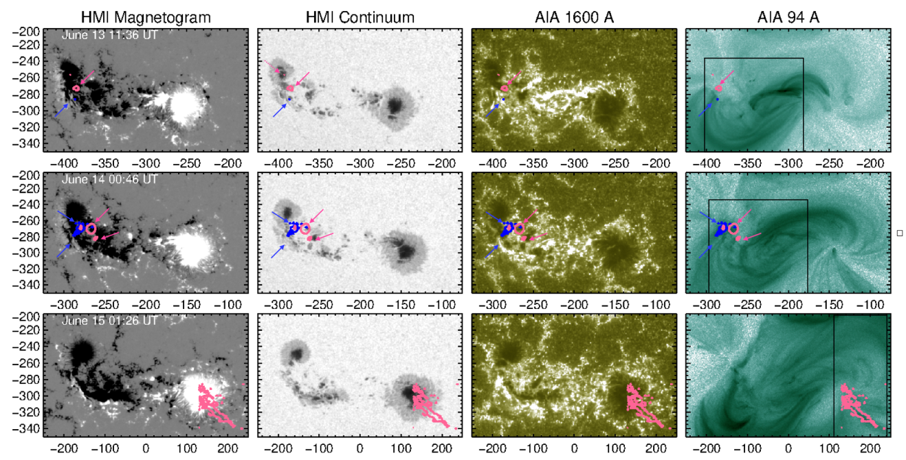
Figure 2: SDO/HMI and AIA observations of AR 11504 on 13 June 2012 at 11:36 UT (top), 14 June at 00:46 UT (middle), and 15 June at 01:26 UT (bottom). Left to right: SDO/HMI line-of-sight magnetogram, SDO/HMI continuum, SDO/AIA 1600 A, and SDO/AIA reverse-color 94 A maps. Contours (and arrows) are of I-FIP from the corresponding Ar XI 188.82 A/Fe XIV 264.79 A (pink) and Ar XIV 194.40 A/Ca XIV 193.87 A (blue) EIS ratio maps in Figure 1. Black boxes in the right column show the approximate EIS FOV for each raster.
Relating Hinode/EIS Observations to the Ponderomotive Force Fractionation Mechanism
Laming (2015) proposed the ponderomotive force associated with Alfvenic waves as the fractionation mechanism that separates ions from neutrals in the chromosphere leading to the well-known FIP effect. The ponderomotive acceleration is proportional to the gradient of delta E2/B2, where delta E is the wave electric field and B is the ambient magnetic field. Since the magnetic field strength usually decreases with height, the upward gradient of delta E2/B2 is generally positive which produces the FIP effect; a negative gradient results in I-FIP plasma.
In the case of the I-FIP effect, fast mode waves originating at/below the fractionation region in the chromosphere undergo total internal reflection and refract back downwards in the lower chromosphere where the Alfvén speed is increasing with height (i.e. the wave amplitude increases with decreasing density; Laming 2021). It is this total internal reflection of waves that provides the downward pointing ponderomotive force in the model. The force acts only on ions, thereby depleting the plasma of the easy to ionize low FIP elements and enhancing the relative abundance of high FIP elements to create the I-FIP effect. The I-FIP effect plasma is then transported to the corona by chromospheric evaporation during flaring.
Assuming a sufficiently strong source of fast mode waves from below where high-FIP and low-FIP ions are fractionated in the chromosphere, the simulations of Laming (2021) show that the degree of I-FIP fractionation primarily depends on: 1. how much the magnetic field expands from the photosphere to the corona (expressed as Bcor/Bphoto), and 2. the ionization balance of key elements in the lower chromosphere. For the case of minimal expansion in the magnetic field (Bcor/Bphoto = 0.7), low FIP elements, including Fe and Ca, and intermediate FIP S were depleted low in the chromosphere just above the plasma beta = 1 layer set at 350 km (see Figure 3 (e,f) of Laming 2021). This is the height at which the perpendicularly propagating fast mode waves were undergoing total internal reflection and creating the negative ponderomotive acceleration. High FIP Ar was unaffected by the downward directed ponderomotive force as it is essentially neutral in the model chromosphere. The Hinode/EIS Ar XIV/Ca XIV and Ar XI/Fe XIV ratio maps are in full agreement with the simulations. The low FIP Ca XIV and Fe XIV are depleted relative to their high FIP Ar ion counterparts. Like Ca and Fe, S is also largely depleted at 4 MK. However, S appears to be only partially depleted at 2 MK. The fractionation of S depends on collisional interactions with the background gas of neutral H, as opposed to ionized H higher up in the chromosphere. The fact that S is fractionated i.e. behaves like a low-FIP element suggests that the height of plasma fractionation is low in the chromosphere or even in the photosphere/subsurface.
The I-FIP effect plasma observed by EIS in AR 11504 is consistent with the predictions of the ponderomotive force fractionation model, suggesting that there is a source of fast-mode waves originating from below the fractionation region in the chromosphere. A candidate for the origin of the required fast mode waves is subchromospheric reconnection. Such waves are spatially localized in magnetic flux tubes and are more likely to have sufficient wave amplitude to cause the fractionation, in contrast to much lower amplitude acoustic waves excited by convective motions that are present everywhere in the chromosphere (Laming 2021).
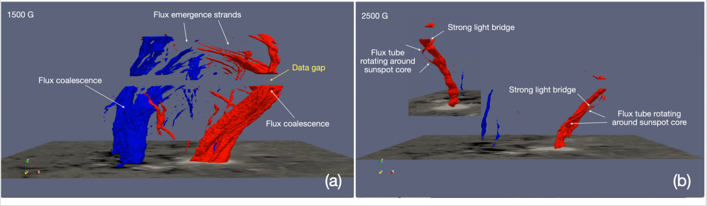
Figure 3: 3D visualization of the subsurface magnetic structure of AR 11504 constructed from stacking contours at 1500 G (a) and 2500 G (b) from the Br component of SHARP vector magnetograms using the method of Chintzoglou & Zhang (2013). Time runs from 17:00 UT on 9 June (top) to 13:00 UT on 20 June (bottom) of each image. Inset in (b) shows the rotating flux tube around the sunspot core of the positive polarity from a different viewing angle. Key locations for subsurface reconnection to take place are: 1. flux coalescence in the following (blue) polarity and 2. at the strong light bridge in the leading (red, positive) polarity.
.
Search for Conditions and Signatures of Subchromospheric Reconnection
We attempt to search for signatures of heating and photospheric upflows as a consequence of subchromospheric reconnection at the places where flux emergence is bringing magnetic flux tubes together, e.g. in merging umbrae, and in particular when new flux is approaching and wrapping around old flux, forming a prominent light bridge, as we observe in the big leading spot of this AR. Light bridges are interfaces between magnetic flux tubes, and in case there is a non-zero angle between the same-polarity magnetic fields being pushed together by ongoing flux emergence, they are likely locations for reconnection below the fractionation region (Toriumi et al, 2015a,b). Knowledge of the subsurface structure of AR 11504 helps to identify potential locatons of subchromospheric reconnection.
The subsurface structure of AR 11504 can be inferred from observations using the image-stacking technique of Chintzoglou & Zhang (2013). A 3D data cube is constructed from SDO/HMI Space-weather HMI Active Region Patches (SHARPs; Bobra et al. 2014) vector magnetograms. The starting time, t0, is at the top of the data cube and the 2D magnetograms forming the X-Y plane are added at progressively lower 'heights' in the Z-direction. Contours of radial magnetic field, Br, from each magnetogram are then stacked along the time dimension. The overall picture from this analysis is an approximation of the sub-photospheric 3D magnetic flux structure at time t0 as it would result from a purely solid-body (kinematic) emergence. The visualization of the 3D structure of AR 11504 from 9-20 June 2012 is displayed in Figure 3. Contour levels of 1500 G and 2500 G (Figure 3(a,b)) were selected to highlight different features of the emerging structure. These are annoted in the figure.
From continuum images, it is clear that light bridges formed as individual flux tubes rotated around the core of the leading sunspot. One of the main light bridges is indicated in the red Br stack in the upper right panel of Figure 3(b) and corresponds to the light bridge of the positive polarity evident in the continuum image of Figure 2(b). I-FIP is observed in the EIS ratio maps on 15 June precisely above this light bridge separating the rotating flux tubes. Furthermore, the loops containing I-FIP plasma appear to be rooted very close to the light bridge (Figure 2). The region of large scale flux emergence mentioned above is highlighted in the negative/following polarity (blue) in Figure 3(a). Before the data gap on June 13, numerous individual strands of emerging flux are clearly identifiable in the following sunspot(s) unlike in the more coherent leading one. After the data gap, the flux emergence has stopped in the south/southeastern section of the AR and the flux has coalesced to form two coherent (blue, negative polarity) sunspots. This is the location where I-FIP was observed on 13 and 14 June while flux emergence/coalescence was taking place. These light bridges are locations where the conditions are possible for subphotospheric reconnection to take place.
Though the 3D visualization of the subsurface structure does not tell us whether reconnection has taken place below the photosphere. it does however, provide a road map of potential locations. We found subtle observational evidence of the consequences of reconnection - outflows and heating.
The top panel of Figure 4 (a,b,c) shows signatures of subchromospheric reconnection outflows in SDO/HMI (photospheric) Dopplergrams. Blue-shifted episodic upflow events along the light bridge are potential tracers of subchromospheric reconnection outflows. There is only one clear upflow event seen along the light bridge in AR 11504. This upflow is shown in Figure 4(c,d). It is seen for about 2 hours (on June 13 between 19:10-21:22 UT), around the time of the formation of the light bridge.
Signatures of heating potentially resulting from subchromospheric reconnection are visible in running-difference (RD) images of co-aligned SDO/HMI continuum, SDO/AIA 1700 and 1600 A images (bottom panels of Figure 4). In the continuum RD image, the light bridge is clearly seen as a black-and-white patterned sharp feature. At 1700 A it is still discernible, but in 1600 A it is not evident at all. As the atmospheric layers these images sample are increasing in height from continuum to 1600 A, it gives a hint of low-altitude weak energy release being present along the light bridge in the photosphere, which then wanes in the lower atmosphere. The light bridge is particularly prominent at its formation on June 13 and increased brightness seems to be present in the vicinity of the upflow event observed in the Dopplergrams.
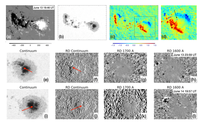
Figure 4: Photospheric observations. HMI LOS magnetogram, (a), continuum intensity (b), Dopplergram (c) and zoomed Dopplergram of boxed region (d). The color scales are in Gauss for the magnetic field and in km/s for the velocity. In panel (d), the black arrow indicates strong upflows at the light bridge. The two lower rows show SDO/HMI continuum, running difference (RD) continuum, RD AIA 1700 A and RD 1600 A images at 23:59 UT on 13 June (e-h) and 19:57 UT on 14 June (i-l). Red arrows point out the ridges of brightenings along the light bridge formed by the coalescence of the leading polarity sunspot. These ridges are not evident in the cospatial/cotemporal SDO/AIA images of the upper photosphere and transition region (panels g,h,k,l).
The horizontal magnetic field in the leading sunspot shows small antiparallel field components on either side of the light bridge on June 14 (see Figure 5(a)). On June 15, closer in time to the I-FIP observation in the leading spot, the horizontal field direction is parallel on either side of the light bridge (see Figure 5(b)). It is interesting to note that if the magnetic field we observe in Figure 3(a,b) is comparable to the field destroyed by reconnection, we can estimate whether there is enough energy for I-FIP fractionation to result from reconnection. When the magnetic energy at 1500 G is converted into waves at a plasma density of 10^17/cm^3, then the wave amplitude is approximately 10 km/s. This level of wave amplitude is of the right order to produce the I-FIP effect according to the ponderomotive force fractionation model.
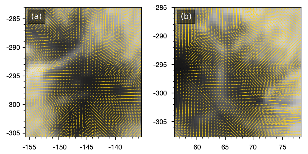
Figure 5: White light continuum images of the leading positive sunspot on (a) 14 June 2012 at 00:58 UT and (b) 15 June at 00:58 UT with arrows that represent the strength and direction of the horizontal magnetic field. In panel (a), the horizontal field on either side of the light bridge (approx x = -147", y = -292") has small antiparallel components with very weak horizontal field in the center of the light bridge. In panel (b), the horizontal field is parallel on either side of the light bridge, but the horizontal field is weaker in the middle of the light bridge (approx x = 64", y = -299").
.
Conclusions
Direct observational evidence of subchromospheric reconnection remains elusive, however, a preponderance of indirect evidence has contributed to our understanding of the conditions required for it to take place and consequences of the processes associated with it. In AR 11504, there were signs of subtle heating and weak short-lived reconnection outflows observed in the photosphere. They were all localized in, or at least nearby, light bridges / in between magnetic flux tubes at the photospheric level.
For more details, see:
Baker et al., accepted ApJ, 2024:
Searching for evidence of subchromospheric magnetic reconnection on the Sun
References
James, A. W., et al. 2017, Sol Phys, 292:71
James, A. W., et al. 2020, A&A, 644:137
Baker, D., et al. 2019, ApJ, 875:35
Baker, D., et al. 2020, ApJ, 874:35
Laming, J. M., 2015, LRSP, 12:2
Laming, J. M., 2021, ApJ, 909:17
Chintzoglou, G. & Zhang, J., 2013, ApJ, 764:L3
Bobra, M. G., et al. 2014, Sol Phys, 289:3549
Touriumi, S., et al. 2015a, ApJ, 811:138
Toriumi, S., et al. 2015b, ApJ, 811:137
Next EIS Nugget »» coming soon...
TBC
Last Revised: 27-Oct-2011
Feedback and comments: webmaster
|