Directly Comparing Coronal and Solar Wind Elemental Fractionation
David Stansby - UCL/MSSL

One key goal for the recently launched Solar Orbiter mission is pinning down the regions of the Sun responsible for producing the solar wind. This means that Solar Orbiter has a large instrument payload, with a combination of remote sensing and in-situ instruments. One proposed method for identifying regions of the solar wind involves simultaneously measuring and comparing the elemental composition of the solar corona and solar wind. Solar Orbiter will be able to do this at high spatial and temporal resolution with the SPICE spectrometer and SWA/HIS heavy ion sensor. However, it is already possible to try this method with the Hinode/EIS spectrometer and ACE/SWICS heavy ion sensor. In this study we performed a direct comparison of coronal and solar wind composition, to understand how the method works and what we will be able to learn with Solar Orbiter.
To get measurements of the composition in the corona we used a full Sun spectrographic observation taken by Hinode/EIS. From this a map of the Silicon/Sulphur (SI/S) abundance was made, which was previously studied in Brooks et al. 2015 (Nat Comms). This was complemented by magnetic field modelling to identify regions of open magnetic field that could contribute to the solar wind. This is shown in Figure 1; for the time period of interest two coronal hole and one active region source region were identified.
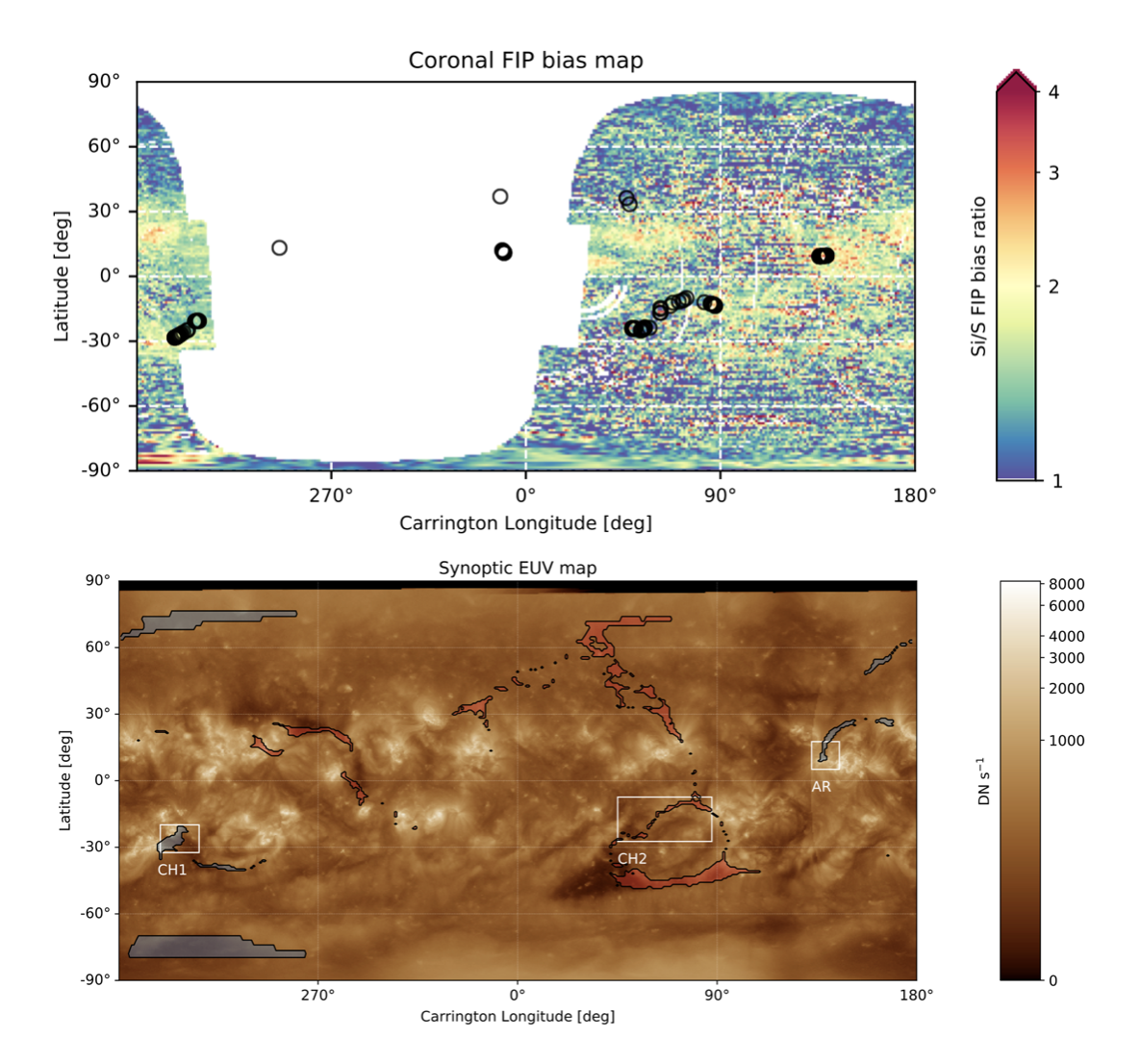
Figure 1: Top panel shows a coronal FIP bias map, with solar wind footpoints denoted as black circles. Bottom panel shows an SDO/AIA 193 synoptic map, with open field regions shown in red/blue shading, and the three solar wind source regions identified with white text and boxes.
To get measurements of the composition in the solar wind we used measurements from the ACE/SWICS instrument. Unfortunately Si/S measurements were not available for the same time period, so we used Iron/Oxygen (Fe/O) measurements instead. Both Si/S and Fe/O are the ratio of a low first ionisation potential (FIP) element to a high FIP element, so both provide a proxy for the FIP bias ratio.
Once we had the solar wind composition, and the coronal composition at the corresponding footpoints, we could make a direct comparison between the two. We found that on small (hourly) timescales there was poor correlation between coronal and solar wind composition (see Figure 3 of the paper), but on the scale of individual source regions the distribution of coronal and solar wind composition values are well matched (see Figure 2 below).
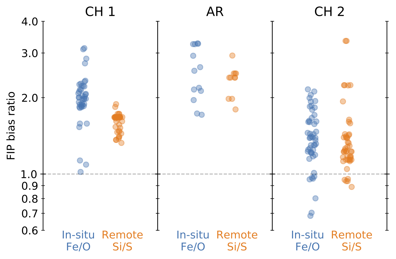
Figure 2: Comparison between coronal and solar wind FIP bias ratio in three different solar wind streams.
From our results we concluded that:
- The matching composition distributions directly verify that elemental composition is conserved as the plasma travels from the corona to the solar wind, validating it as a tracer of heating and acceleration processes.
- It is not possible to identify solar wind source regions solely by comparing solar wind and coronal composition measurements, since there is an overlap in the distribution of composition measurements between different sources.
- A comparison between coronal and solar wind composition can be used to verify consistency with predicted spacecraft-corona connections.
For more details, see Stansby et al. (2020a), A&A:
Directly comparing coronal and solar wind elemental fractionation
References
Brooks, D. H., Ugarte-Urra, Ignacio, Warren, H. P. 2015, Nature Communications, 6, 5947
Next EIS Nugget »» coming soon...
TBC
Last Revised: 27-Oct-2011
Feedback and comments: webmaster
|