Atmospheric Response of an Active Region to new Small Flux Emergence
David Shelton, Louise Harra, Lucie Green (UCL-MSSL)

This study looks at an emerging flux region (EFR) to determine how a small flux emergence event affects the pre-existing active region into which it emerges. In many cases, the magnetic flux emerges as a fragmented structure called the serpentine field. If magnetic reconnection does facilitate the emergence of the serpentine field into the atmosphere, we should see some evidence for this in the form of brightenings, jets, new loops and upflow/downflow enhancements.
In Shelton et al. (2015) we investigate the atmospheric responses to a small emerging flux region that was seen on the solar surface from 23 June 2011 to 25 June 2011. We show that coronal jets can form in the serpentine field, that the magnetic field can move across an active region and that this can allow loops to form away from the EFR even on small-scales.
Results and Discussion
The first coronal jets are seen in the AIA 193 Å wavelength channel approximately four minutes after the first chromospheric jets. There are no coronal jets seen over this region before the flux emergence begins. They are spatially located over the region of magnetic flux emergence with the footpoints appearing to be in the serpentine field rather than at the major polarities of the EFR. This is the first time that coronal jets have ever been seen over any serpentine. The chromospheric and coronal jets are seen over the serpentine from approximately two hours after the start of the serpentine emergence until the end of the serpentine emergence. This has not been seen before and this is possibly due to the lack of high temporal and spatial resolution. This tells us that the emerging serpentine field can release the energy required to produce jets and heat the corona.
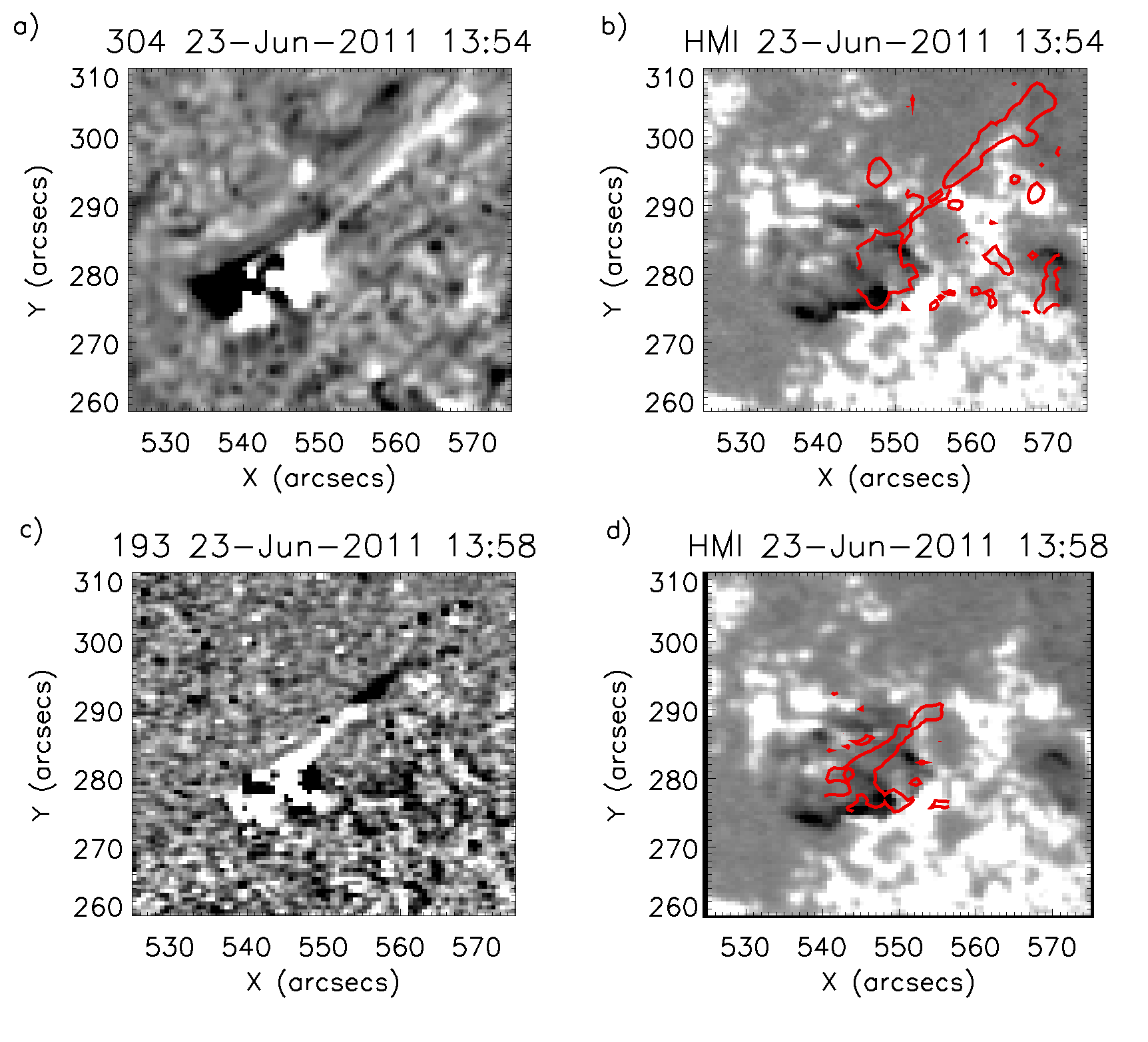
Figure 1: The first jets seen in the chromosphere (304 Å) and corona (193 Å) five hours after the flux emergence begins. (a): A running difference AIA 304 Å intensity map of the jet between 13:48 and 13:54 (the image from 13:48 is removed from the image at 13:54) on 23 June 2011. (b): The closest HMI image to when the 304 Å jet is released. The red contours in (a) and (b) show the location of the jet seen in the 304 Å difference image. (c): A running difference AIA 193 Å intensity map of the jet between 13:58 and 14:02 (the image from 13:58 is removed from the image at 14:02) on 23 June 2011. (d): The closest HMI image to when the 193 Å jet is released. The red contours in (c) and (d) show the location of the jet seen in the 193 Å difference image.
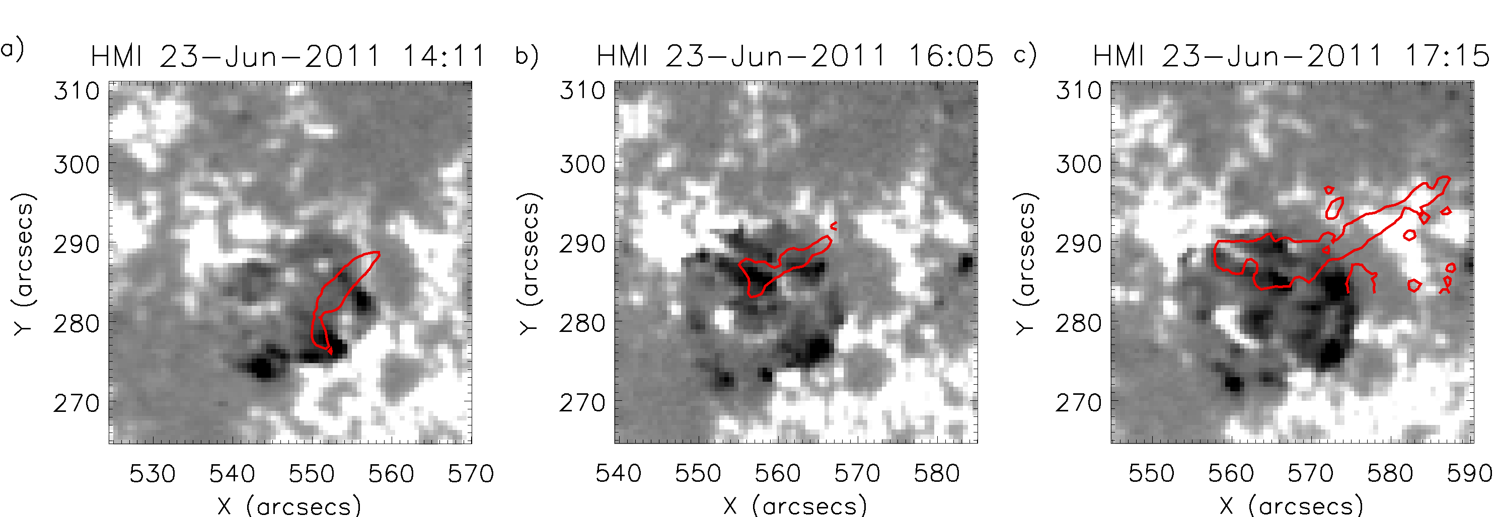
Figure 2: Jets seen migrating across the serpentine field. The contours show the jets. The jets start at the boundary between the flux emergence and the pre-existing active region (a), then move to the centre of the flux emergence (b) and then move to the north boundary between the flux emergence and the pre-existing active region (c).
As the serpentine emerges, the jets appear to move across the flux emergence towards the north part of the EFR. The jets start at the boundary between the flux emergence and the pre-existing active region, then start forming over the serpentine field, before forming over the boundary between the flux emergence and pre-existing active region in the north. After this, the serpentine field has fully emerged and jets form between the large-scale EFR field and the pre-existing active region. These jets form at the EFR's south boundary with the pre-existing active region and last for 5 hours.
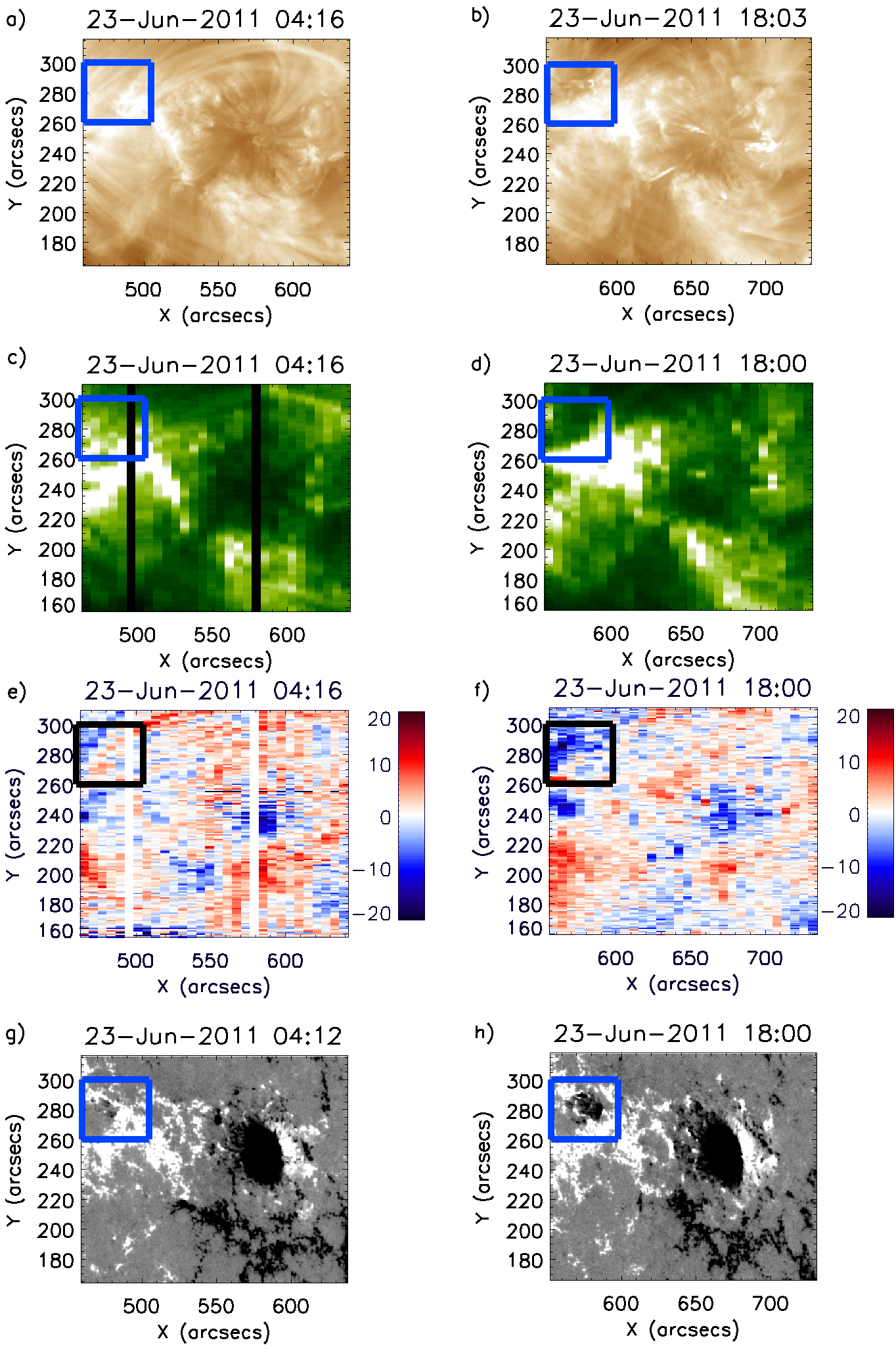
Figure 3: Figure 3 caption: (a) and (b): AIA 193 Å intensity maps before (five hours) and after (nine hours) the flux emergence begins. (c) and (d): Shows EIS Fe XII intensity maps before (five hours) and after (nine hours) the flux emergence begins. (e) and (f): EIS Fe XII Doppler velocity maps before (five hours) and after (nine hours) the flux emergence begins. The Doppler velocity range is between +/-20 km/s. (g) and (h): two HMI magnetogram maps before (five hours) and after (nine hours) the flux emergence begins. The minimum magnetic field strength is +/-25 G. The boxes show where the new flux region will emerge.
In the EIS velocity maps, blueshift enhancements are seen after the magnetic flux emergence begins, and there is also an intensity enhancement in the EIS intensity maps after the magnetic flux emergence begins. These enhancements were not seen before the magnetic flux emergence. The blueshifts are located where positive and negative flux meet at the north part of the EFR and where there are intensity enhancements in the EIS 195 Å data. We compared the upflow velocities before and during the flux emergence in Figure 3 and we find that there is an average upflow velocity enhancement of 10 +/-4 km/s.
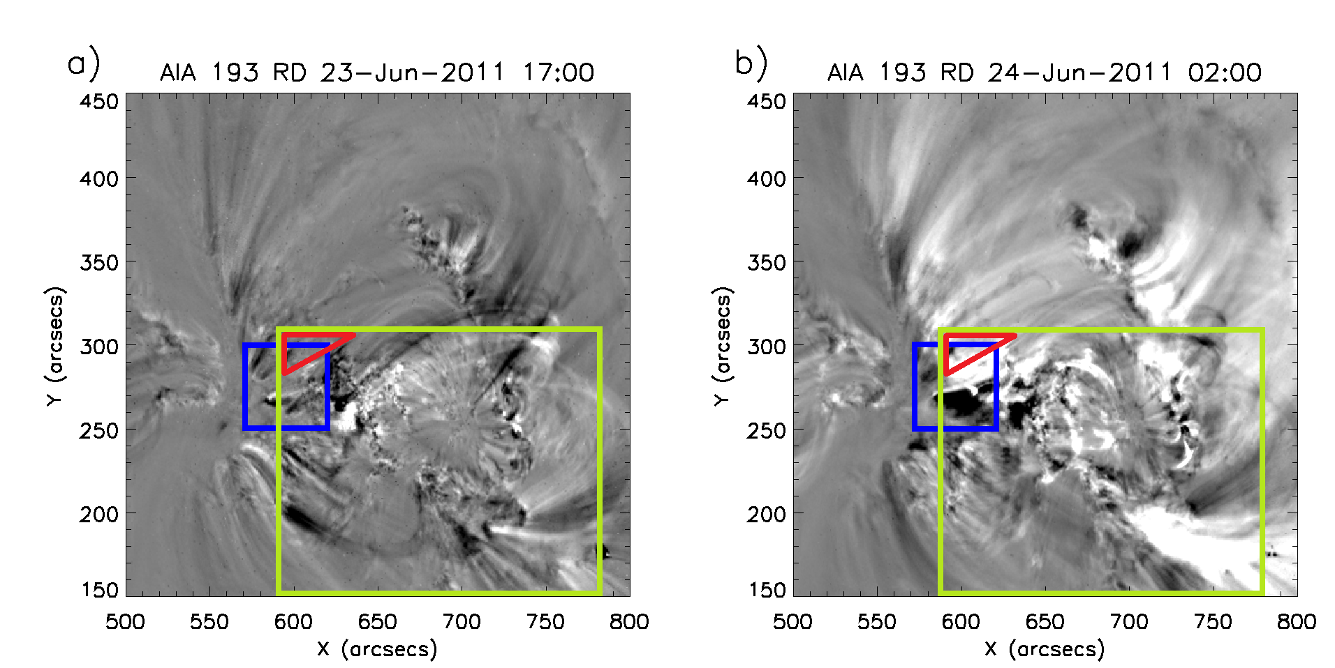
Figure 4: Running difference images before the rise in intensity (a) and at the peak of the intensity rise (b). We can clearly see an enhancement in intensity to the north of the EFR (highlighted by the small box). The large box represents the EIS field of view and the triangle represents the area in which we see the upflow enhancements.
It can be seen that the enhanced blueshifts are located in the northern part of the EFR which is associated with the lower legs of the large-scale loops. This suggests that the cause of the blueshifts is chromospheric evaporation. These large-scale loops continue to exist after the emergence phase has ended and form 43 Mm away from the emerging flux. It is possible for coronal jets to form over the serpentine field as the serpentine field is emerging. The jets are also seen to migrate across the serpentine via interchange reconnection. After the serpentine field has fully emerged, jets are seen forming over the large-scale EFR field.
References
Shelton, D., Harra, L., Green, L., 2015, Sol. Phys., 290, 753.
Next EIS Nugget »» coming later...
TBC
Last Revised: 16-Dec-2015
Feedback and comments: webmaster
|