EIS radiometric calibration#
UPDATE, 13-May-2025: All EIS users are now recommended to use the calibration described in Del Zanna et al. (2025, ApJS, 276, 42) . See below under "The 2025 update".
Lang et al. (2006) described the laboratory calibration of EIS and this is implemented by eis_prep. For the period 2011-2013 EIS users were recommended to use the /correct_sensitivity when calling eis_prep, which implemented an exponential sensitivity decay as a function of time that was uniformly applied to all wavelengths.
Re-assessments of the EIS calibration were performed independently by G. Del Zanna and H. Warren around 2013-2014, and these are described below along with software routines that implement the calibrations. These two authors collaborated to yield the new calibration in 2025.
The recommendation for users is to run eis_prep with the default options, yielding intensities computed with the original laboratory calibration. The intensities can then be modified to the newer calibrations as described below.
Users are encouraged to report to the EIS team any problems that result from using the new calibrations.
The 2025 update#
The 2025 calibration is implemented through the routine interpol_eis_ea. The following call shows how to generate the effective area on 1-May-2020 for the EIS SW channel:
IDL> wvl=findgen(41)+170.
IDL> ea=interpol_eis_ea('1-may-2020',wvl
There is also the routine eis_recalibrate_intensity_new that is useful for converting an intensity from the original laboratory calibration to the new calibration. For example, if the old intensity for the 195.12 line was 100, then the new intensity is given by
IDL> int=eis_recalibrate_intensity_new('1-may-2020',195.12,100.)
If you use the routines EIS_AUTO_FIT and/or EIS_MASK_SPECTRUM, then see the instructions at the bottom of this page.
G. Del Zanna method (2013)#
This method is described in Del Zanna (2013). If you derived a line intensity with the original lab calibration, then the corrected intensity is derived by multiplying by the factor
IDL> cal_factor=eis_ltds(date,wvl)
where 'date' is the observation date and 'wvl' is the wavelength.
If you had previously used the /correct_sensitivity option in eis_prep, then the correction factor is given by:
IDL> cal_factor=eis_ltds(date,wvl,/undecay)
Warren, Ugarte-Urra, and Landi method (2014)#
We have attempted to extend Giulio's method of using the atomic data to infer the shape of the effective areas by including information from the SDO/EVE instrument. EIS routinely makes full-disk mosaics (HOP130), which can be used to compute irradiances that be compared with those from EVE. Below is a comparison of the EIS and EVE irradiances for 195.
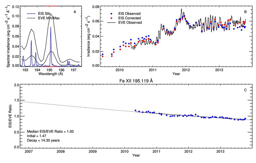 |
We then use very deep observations taken above the limb to fit a model that includes both an emission measure distribution and potential modifications to the effective areas. The effective area near 195 is fixed to lie on the EIS-EVE curve shown above. Here is an example of this applied to some off-limb spectra taken in 2007.
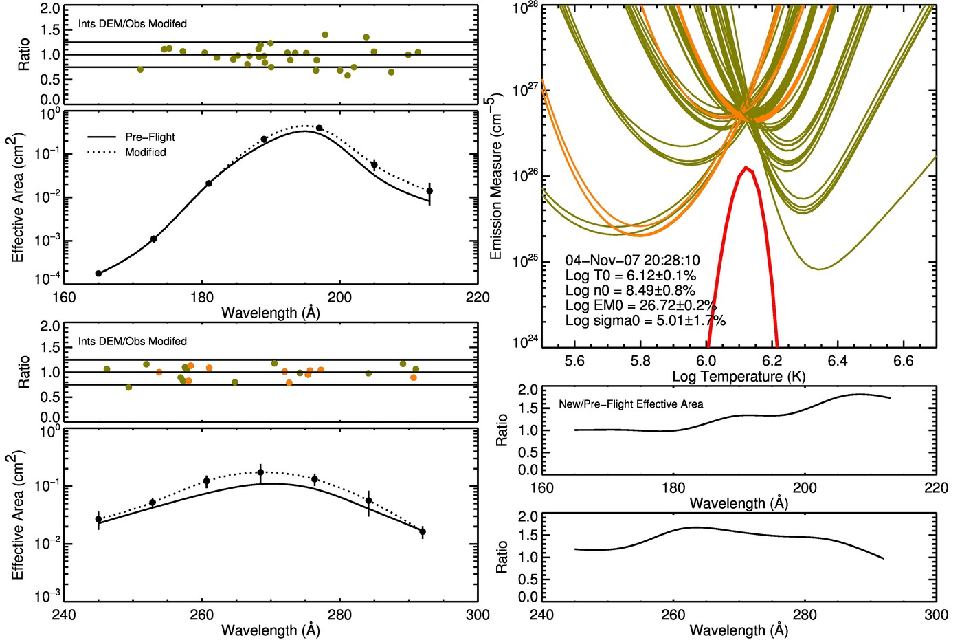 |
By repeating this analysis for several periods during the mission we are able to infer the effective areas as a function of wavelength and time. Details are given in the paper Warren, Ugarte-Urra & Landi (2014).
There is software distributed in SSW that computes the new effective areas. Perhaps the most useful routine is eis_recalibrate_intensity.pro which takes an intensity computed with the pre-flight calibration and computes the corresponding intensity for the modified effective areas. One can also use eis_ea_nrl to compute the new effective areas as a function of wavelength and time.
Checking the calibration status of your existing data#
If you have level-1 data on your computer for which you'd like to apply the new calibrations, but you can't remember whether you used the /correct_sensitivity keyword or not, then do:
IDL> d=obj_new("eis_data", eis_file)
IDL> print,(d->getcalstat()).sens
The result will be 1 if /correct_sensitivity was used, and 0 otherwise.
If you use the windata structures, then check the value of windata.hdr.cal_sens.
Applying the new calibrations to the output from EIS_AUTO_FIT and EIS_MASK_SPECTRUM#
If you use the Gaussian fitting routine EIS_AUTO_FIT, then the recommendation is to apply the new calibrations at the EIS_GET_FITDATA stage. For example,
IDL> int=eis_get_fitdata(fitdata,/int,calib=1
will apply the Del Zanna (2013) calibration to the output intensity. The options are:
0 - the calibration is not changed
1 - the Del Zanna (2013) calibration is applied
2 - /correct_sensitivity is "undone" and the Del Zanna (2013) calibration is applied
3 - the Warren et al. (2014) calibration is applied
4 - /correct_sensitivity is "undone" and the Warren et al. (2014) calibration is applied
5 - the Del Zanna et al. (2025) calibration is applied
6 - /correct_sensitivity is "undone" and the Del Zanna et al. (2025) calibration is applied
To summarize, the steps to be done are:
- Use EIS_PREP to calibrate the level-0 file with standard options (no /correct_sensitivity).
- Extract the windata structure using EIS_GETWINDATA with the /refill option.
- Perform the Gaussian fit with EIS_AUTO_FIT.
- Extract the intensity array with EIS_GET_FITDATA using the calib option set to 5 (2025 calibration).
Similarly, if you use the routine EIS_MASK_SPECTRUM to derive a spectrum from a pixel mask, then you can specify the calibration using the CALIB= keyword. For example:
IDL> eis_mask_spectrum,file,mask,swspec=swspec,lwspec=lwspec,calib=5,/refill